Current Method in Literature :
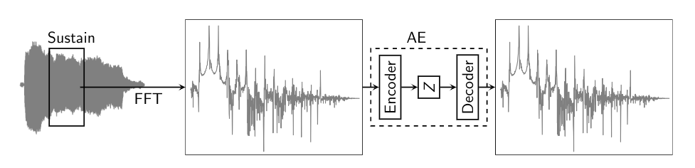
The above framewise log-magnitude spectra reconstruction procedure is described in [1]. We implemented it as shown using an Autoencoder, and observe that the reconstruction cannot generalize to pitches the network has not been trained on. For demonstration, we train the network including and excluding MIDI 63 along with its 3 neighbouring pitches on either side :
(a) Including MIDI 63
| MIDI | 60 | 61 | 62 | 63 | 64 | 65 | 66 |
|---|---|---|---|---|---|---|---|
| Kept | $\checkmark$ | $\checkmark$ | $\checkmark$ | $\checkmark$ | $\checkmark$ | $\checkmark$ | $\checkmark$ |
(b) Excluding MIDI 63
| MIDI | 60 | 61 | 62 | 63 | 64 | 65 | 66 |
|---|---|---|---|---|---|---|---|
| Kept | $\checkmark$ | $\checkmark$ | $\checkmark$ | $\times$ | $\checkmark$ | $\checkmark$ | $\checkmark$ |
We then give MIDI 63 as an input to both the above cases, and see how well the network can reconstruct the input
import IPython.display as ipd
print('Input MIDI 63 Note')
ipd.display(ipd.Audio('./ex/D#_19_og.wav'))
print('(a) Reconstructed MIDI 63 Note when trained Including MIDI 63')
ipd.display(ipd.Audio('./ex/D#_19_trained_recon_stft_AE.wav'))
print('(b) Reconstructed MIDI 63 Note when trained Excluding MIDI 63')
ipd.display(ipd.Audio('./ex/D#_19_skipped_recon_stft_AE.wav'))
%%HTML
<a href="./ex/Ds_19_og.png" target="_blank">Input MIDI 63 Spectrogram</a> <br>
<a href="./ex/Ds_19_trained_recon.png" target="_blank">(a) Reconstructed MIDI 63 Spectrogram when trained Including MIDI 63</a> <br>
<a href="./ex/Ds_19_skipped_recon.png" target="_blank">(b) Reconstructed MIDI 63 Spectrogram when trained Excluding MIDI 63</a> <br>
On hearing the reconstructed version of the input note, and looking at the spectrograms, you can clearly see that the frame-wise magnitude spectrum based reconstruction procedure cannot reconstruct pitches it has not been trained on. This gives us a good motivation to move on to a parametric model
Proposed Method
Parametric Model
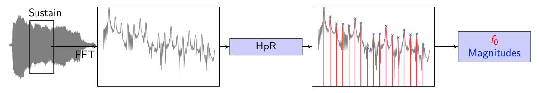
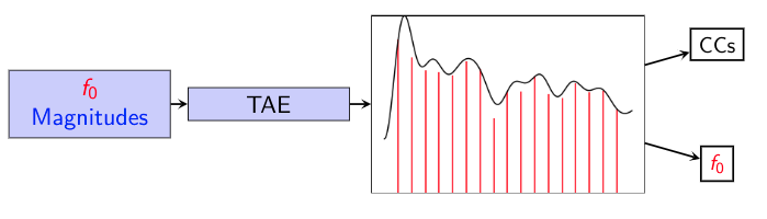 The above shows the Parametric(Source-Filter) representation of a signal. The procedure is described in detail in [2]. The TAE algorithm is described in [3].
The audio clip below show the Parametric reconstruction of an input audio note. As mentioned in the paper, we only work with the harmonic component, and neglect the residual for now
print('Original MIDI 60 Note')
ipd.display(ipd.Audio('./ex/C_3.wav'))
print('Source Filter Reconstructed MIDI 60 Note')
ipd.display(ipd.Audio('./ex/C_3_recon.wav'))
# print('Original F4 Note')
# ipd.display(ipd.Audio('./Audio_SF/F_15.wav'))
# print('Source Filter Reconstructed F4 Note')
# ipd.display(ipd.Audio('./Audio_SF/F_15_recon.wav'))
# print('Original B4 Note')
# ipd.display(ipd.Audio('./Audio_SF/B_15.wav'))
# print('Source Filter Reconstructed B4 Note')
# ipd.display(ipd.Audio('./Audio_SF/B_15_recon.wav'))
Network Architecture
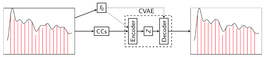
This is our proposed model - VaPar Synth - a Variational Parametric Synthesizer which utilizes a Conditional Variational Autoencoder(CVAE) trained on the parametric representation.
We demonstrate the experiments performed ahead.
Experiments
Experiment 1 - Reconstruction
The table below shows training when skipping MIDI 63, and training on its 3 nearest neighbours.
| MIDI | 60 | 61 | 62 | 63 | 64 | 65 | 66 |
|---|---|---|---|---|---|---|---|
| Kept | $\checkmark$ | $\checkmark$ | $\checkmark$ | $\times$ | $\checkmark$ | $\checkmark$ | $\checkmark$ |
We show the input note 63, and the reconstructions by the AE and CVAE.
print('Input MIDI 63 Note')
ipd.display(ipd.Audio('./ex/D#_19_input_pm.wav'))
print('AE reconstruction')
ipd.display(ipd.Audio('./ex/D#_19_recon_AE.wav'))
print('CVAE reconstruction')
ipd.display(ipd.Audio('./ex/D#_19_recon_cVAE.wav'))
# %%HTML
# <a href="./ex/Ds_19.png" target="_blank">Spectral Envelope(Input and Reconstruction)</a>
On listening to both the reconstructions, both AE and CVAE can reconstruct the input note inspite of not being trained on that pitch.
We also train our model only on the endpoints, and skip all the other pitches in the octave, as shown in the table below.
| MIDI | 60 | 61 | 62 | 63 | 64 | 65 | 66 | 67 | 68 | 69 | 70 | 71 |
|---|---|---|---|---|---|---|---|---|---|---|---|---|
| Kept | $\checkmark$ | $\times$ | $\times$ | $\times$ | $\times$ | $\times$ | $\times$ | $\times$ | $\times$ | $\times$ | $\times$ | $\checkmark$ |
We show the reconstruction of a pitch which is far away from the train points - MIDI 65, and analyze how the network reconstructs this pitch
print('Input MIDI 65 Note')
ipd.display(ipd.Audio('./ex/F_20_og.wav'))
print('AE reconstruction')
ipd.display(ipd.Audio('./ex/F_20_recon_AE.wav'))
print('CVAE reconstruction')
ipd.display(ipd.Audio('./ex/F_20_recon_cVAE.wav'))
# %%HTML
# <a href="./ex/F_20.png" target="_blank">Spectral Envelope(Input and Reconstruction)</a>
Both AE and CVAE sound 'similar' to the input. More formal listening tests will have to be performed to understand the reconstruction better.
Experiment 2 - Generation
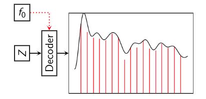
To 'generate' audio from the network, we simply sample points from the latent space, and provide the pitch as a conditional parameter (as shown above).
We train the network on the whole octave sans MIDI 65, and we see how well it can generated MIDI 65. We present both the network generated MIDI 65 note, and a similar MIDI 65 from the dataset.
print('Network Generated MIDI 65 note')
ipd.display(ipd.Audio('./ex/65_gen.wav'))
print('Similar MIDI 65 Note from Dataset')
ipd.display(ipd.Audio('./ex/65_ogg.wav'))
The generated note is missing the soft noisy sound of the violin bowing. This is expected because we only model the harmonic component and neglect the residual.
We have also added a vibrato to the generated note to demonstrate that the network can synthesize continuosly varying frequencies.
print('Network Generated MIDI 65 note with vibrato')
ipd.display(ipd.Audio('./ex/65_gen_vibrato.wav'))
References
- Roche, Fanny, et al. "Autoencoders for music sound modeling: a comparison of linear, shallow, deep, recurrent and variational models." arXiv preprint arXiv:1806.04096 (2018).
- Caetano, Marcelo, and Xavier Rodet. "A source-filter model for musical instrument sound transformation." 2012 IEEE International Conference on Acoustics, Speech and Signal Processing (ICASSP). IEEE, 2012.
- Röbel, Axel, and Xavier Rodet. "Efficient spectral envelope estimation and its application to pitch shifting and envelope preservation." 2005.
%%HTML
<script>
function code_toggle() {
if (code_shown){
$('div.input').hide('500');
$('#toggleButton').val('Show Code')
} else {
$('div.input').show('500');
$('#toggleButton').val('Hide Code')
}
code_shown = !code_shown
}
$( document ).ready(function(){
code_shown=false;
$('div.input').hide()
});
</script>
<form action="javascript:code_toggle()"><input type="submit" id="toggleButton" value="Show Cells"></form>